Cafe Linea things to do, attractions, restaurants, events info and trip planning
Basic Info
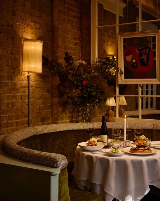
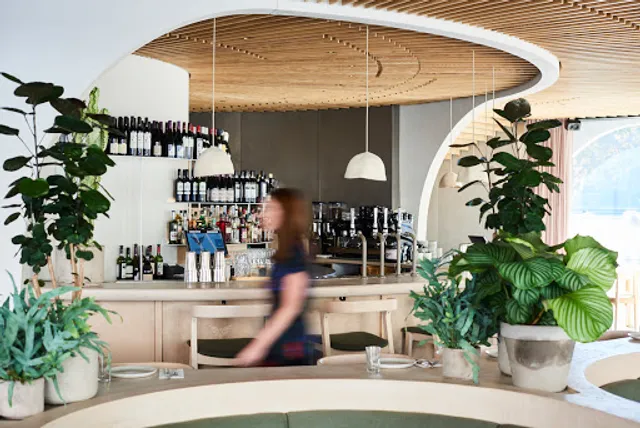
Cafe Linea
90, duke of york square, London SW3 4LY, United Kingdom
4.5(133)
Open until 10:30 PM
Save
spot
spot
Ratings & Description
Info
attractions: Saatchi Gallery, Ever After Garden - Royal Marsden Cancer Charity, Cadogan Hall, The Royal Court Theatre, Venus Fountain, National Army Museum, Royal Hospital Chelsea, Royal Hospital Chelsea Chapel, Chelsea Physic Garden, The Chelsea Pensioners Exhibition, restaurants: POLPO Italian Restaurant Chelsea, Vardo Chelsea, Manicomio, Comptoir Libanais Chelsea, Kutir, The Black Penny | Sloane Square, Côte Sloane Square, Ixchel, Botanist Sloane Square, Colbert, local businesses: Duke of York Square, ZARA, Peter Jones & Partners, John Lewis Sloane Square, Boots, lululemon, John Sandoe (Books) Ltd, Innofinity Worldwide, OFFICE Kings Road, King's Rd
Phone
+44 20 4553 8565
Website
linealondon.com
Open hoursSee all hours
Sat9 AM - 10:30 PMOpen
Plan your stay

Pet-friendly Hotels in London
Find a cozy hotel nearby and make it a full experience.
Affordable Hotels in London
Find a cozy hotel nearby and make it a full experience.
The Coolest Hotels You Haven't Heard Of (Yet)
Find a cozy hotel nearby and make it a full experience.
Trending Stays Worth the Hype in London
Find a cozy hotel nearby and make it a full experience.
Reviews
Live events
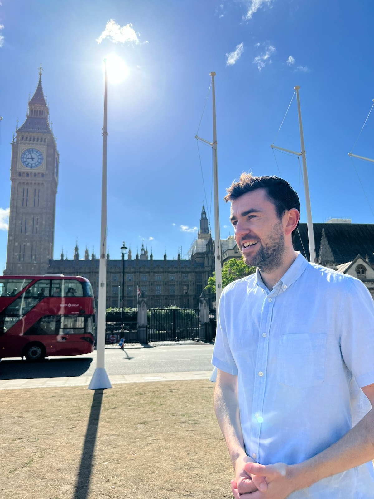
Walk London with a local - in easy English
Sun, Feb 8 • 9:30 AM
Greater London, W1J 9BT, United Kingdom
View details
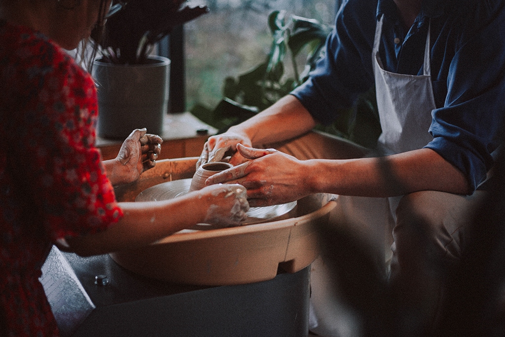
London Pottery Workshop
Sat, Feb 7 • 3:00 PM
Greater London, HA0 1RQ, United Kingdom
View details
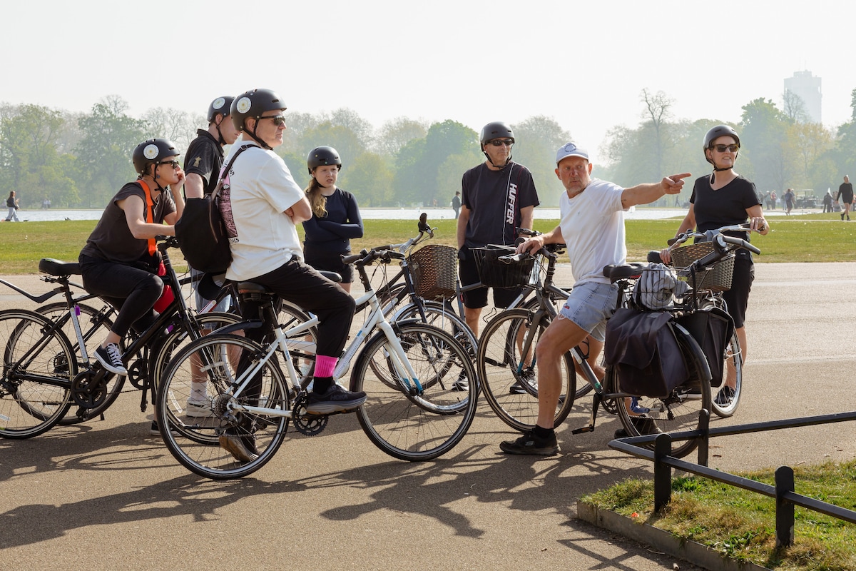
Visit London landmarks and royal parks
Sat, Feb 14 • 10:00 AM
Greater London, W2 4RJ, United Kingdom
View details
Nearby attractions of Cafe Linea
Saatchi Gallery
Ever After Garden - Royal Marsden Cancer Charity
Cadogan Hall
The Royal Court Theatre
Venus Fountain
National Army Museum
Royal Hospital Chelsea
Royal Hospital Chelsea Chapel
Chelsea Physic Garden
The Chelsea Pensioners Exhibition
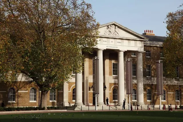
Saatchi Gallery
4.5
(4K)
Open until 6:00 PM
Click for details
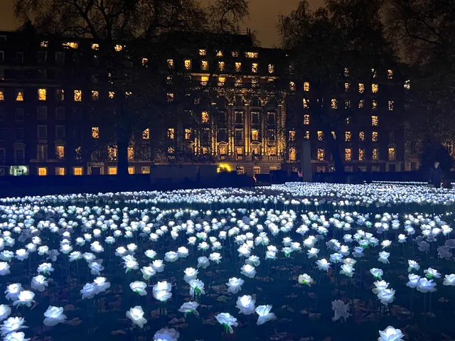
Ever After Garden - Royal Marsden Cancer Charity
4.5
(302)
Open 24 hours
Click for details
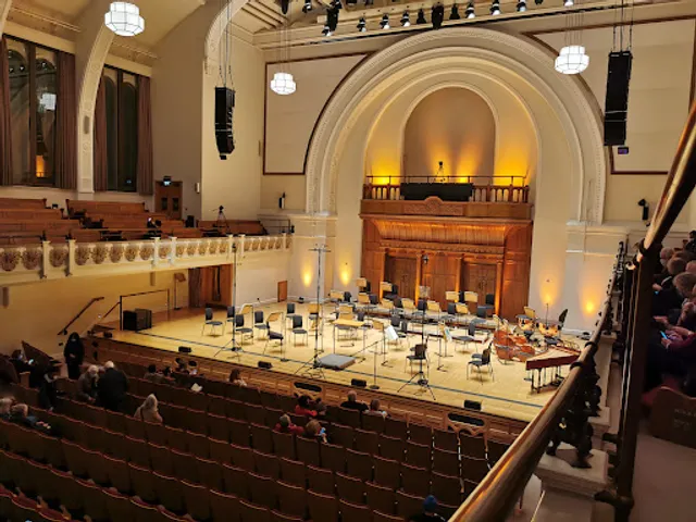
Cadogan Hall
4.7
(1.6K)
Open 24 hours
Click for details
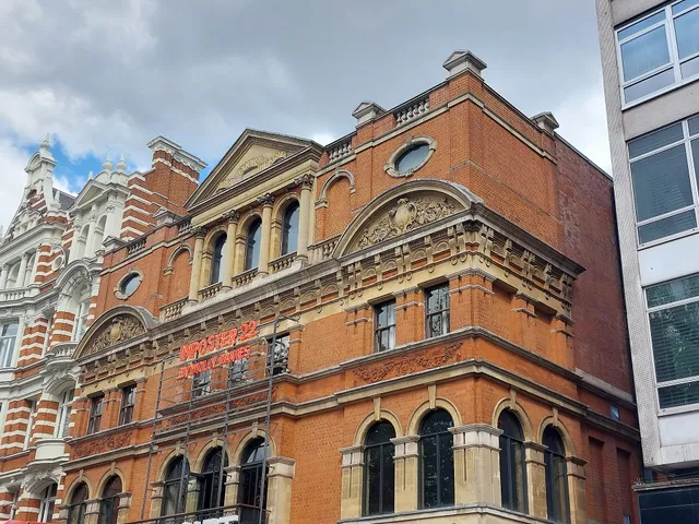
The Royal Court Theatre
4.6
(308)
Open 24 hours
Click for details
Nearby restaurants of Cafe Linea
POLPO Italian Restaurant Chelsea
Vardo Chelsea
Manicomio
Comptoir Libanais Chelsea
Kutir
The Black Penny | Sloane Square
Côte Sloane Square
Ixchel
Botanist Sloane Square
Colbert
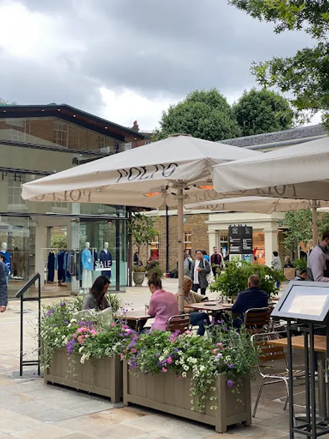
POLPO Italian Restaurant Chelsea
4.3
(742)
$$
Open until 11:00 PM
Click for details
Vardo Chelsea
4.4
(844)
$$
Open until 10:30 PM
Click for details
Manicomio
4.2
(510)
$$$
Open until 12:00 AM
Click for details
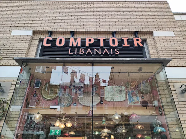
Comptoir Libanais Chelsea
4.1
(954)
Open until 10:00 PM
Click for details
Nearby local services of Cafe Linea
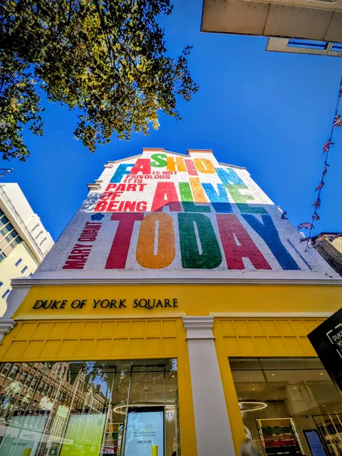
Duke of York Square
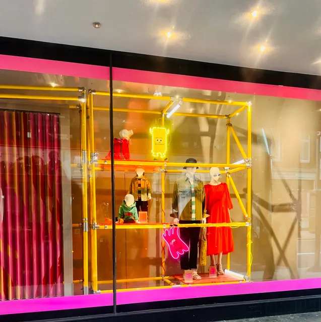
ZARA
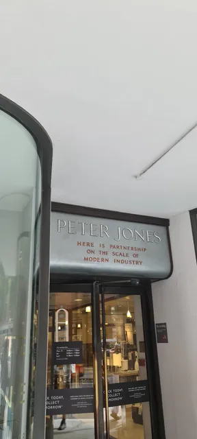
Peter Jones & Partners
John Lewis Sloane Square
Boots
lululemon
John Sandoe (Books) Ltd
Innofinity Worldwide
OFFICE Kings Road
King's Rd
Duke of York Square
4.5
(1.9K)
Click for details
ZARA
4.0
(521)
Click for details
Peter Jones & Partners
4.2
(1.1K)
Click for details
John Lewis Sloane Square
4.4
(374)
Click for details


The hit list


Plan your trip with Wanderboat
Welcome to Wanderboat AI, your AI search for local Eats and Fun, designed to help you explore your city and the world with ease.
Powered by Wanderboat AI trip planner.